CS-466/566: Math for AI

Module 05: Deep Learning Fundamentals-1

Dr. Mahmoud Mahmoud

The University of Alabama

2026-03-23

TABLE OF CONTENTS

1. Introduction●

2. Gates Using Perceptrons○

3. Neural Network as Computational Graph○

4. Automatic Differentiation○

Introduction

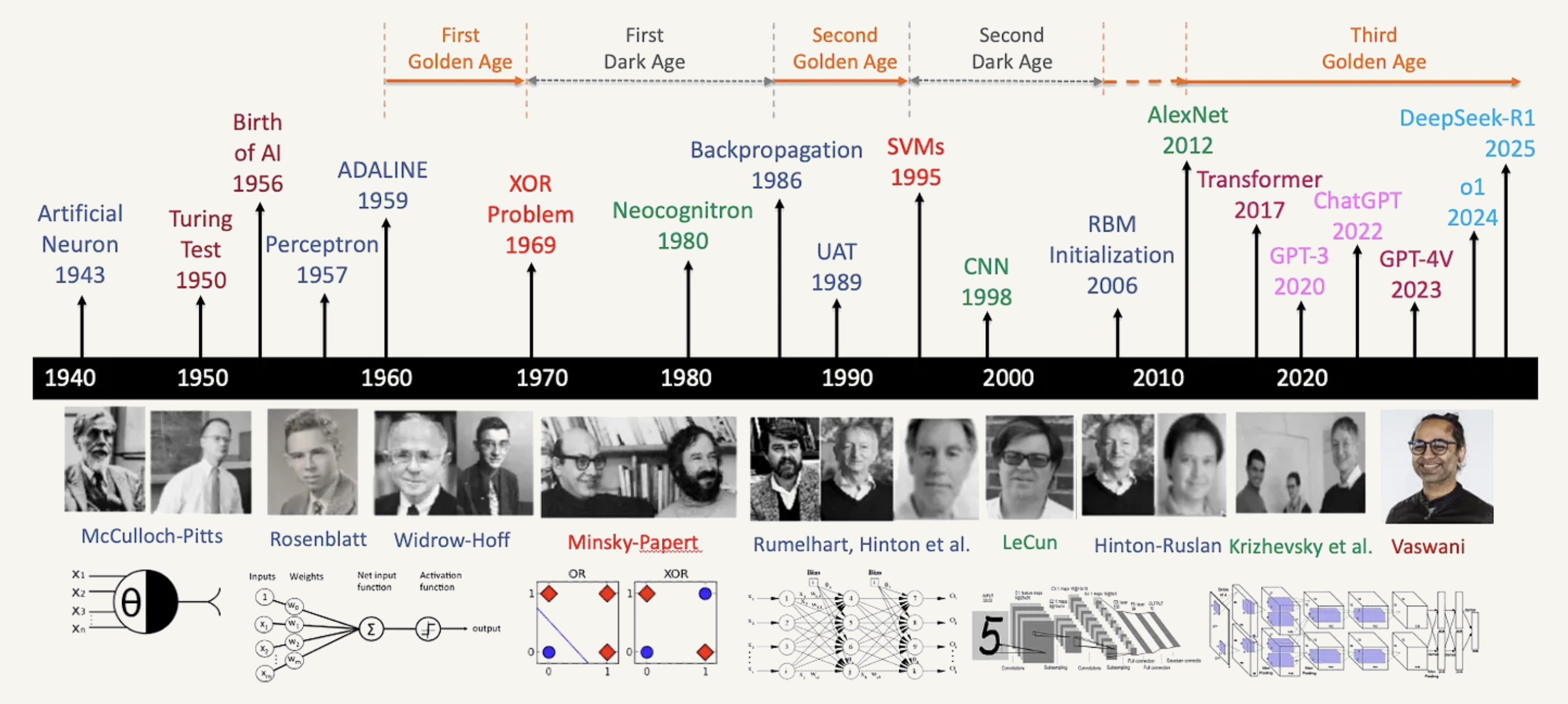
• Goes back to 1940, when people started to build models that imitate the human brain.
• Logistic regression (perceptron) is the core of neural networks started in 1950.
• However, scientists in that time showed that a single perceptron can not solve xor problem (died).
• Reborn in 1980, discovery of merging perceptrons together. But died due to the resources requirements
• Reborn in the last decade with the advancement of the computation resouces.

TABLE OF CONTENTS

1. Introduction✓

2. Gates Using Perceptrons●

3. Neural Network as Computational Graph○

4. Automatic Differentiation○

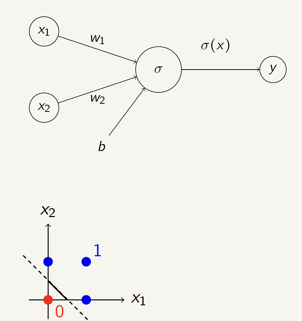
AND Gate Neural Network

Can we build an AND gate using a single perceptron?

\(x_1\)	\(x_2\)	\(y\)
0	0	0
0	1	0
1	0	0
1	1	1

Solution:

\(w_1 = 10\), \(w_2 = 10\), \(b = -15\)

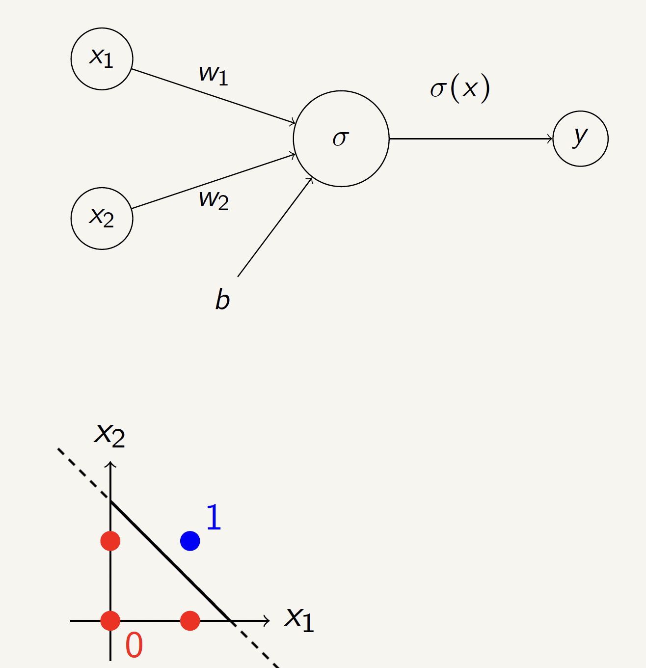
OR Gate Neural Network

Can we build an OR gate using a single perceptron?

\(x_1\)	\(x_2\)	\(y\)
0	0	0
0	1	1
1	0	1
1	1	1

Solution:

\(w_1 = 10\), \(w_2 = 10\), \(b = -5\)

XOR Gate Neural Network

Can we build an XOR gate using a single perceptron?

No! We need multiple layers.

\(x_1\)	\(x_2\)	\(y\)
0	0	0
0	1	1
1	0	1
1	1	0

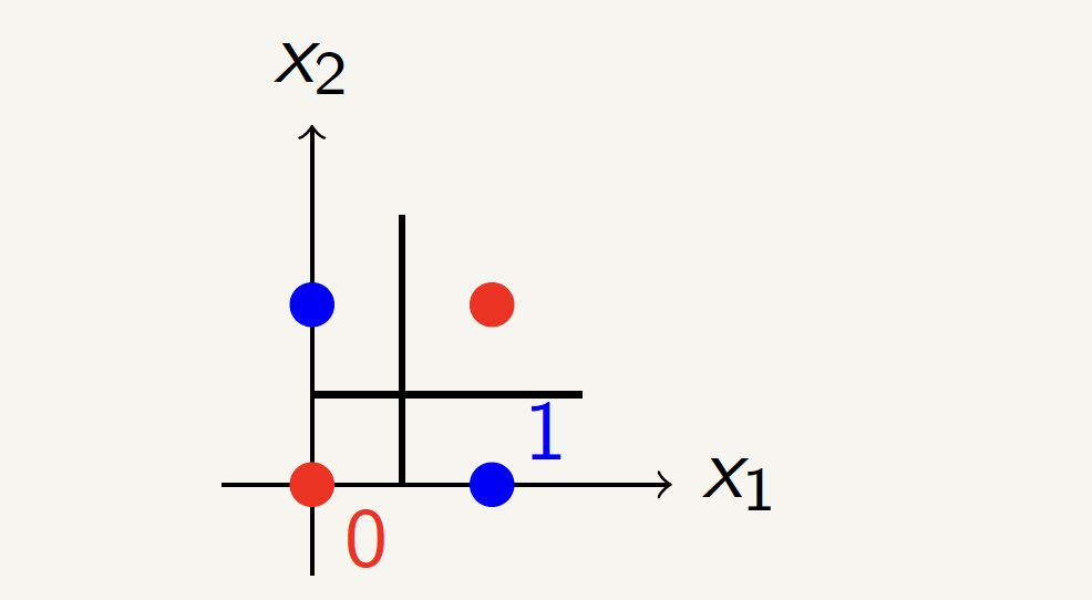
Solving XOR with a Neural Network

Neurons and the Brain

Types of Layers

1. The input layer
Introduces input values into the network. No activation function or other processing.

2. The hidden layer(s)
Perform classification of features. Two hidden layers are sufficient to solve any problem.

3. The output layer
Functionally just like the hidden layers. Outputs are passed on to the world outside the neural network.

Neural Network Design

To train a neural network, we need to find the best values for the weights.

This is done using gradient descent algorithm:

\[W \leftarrow W - \eta \frac{\partial L}{\partial W}\]

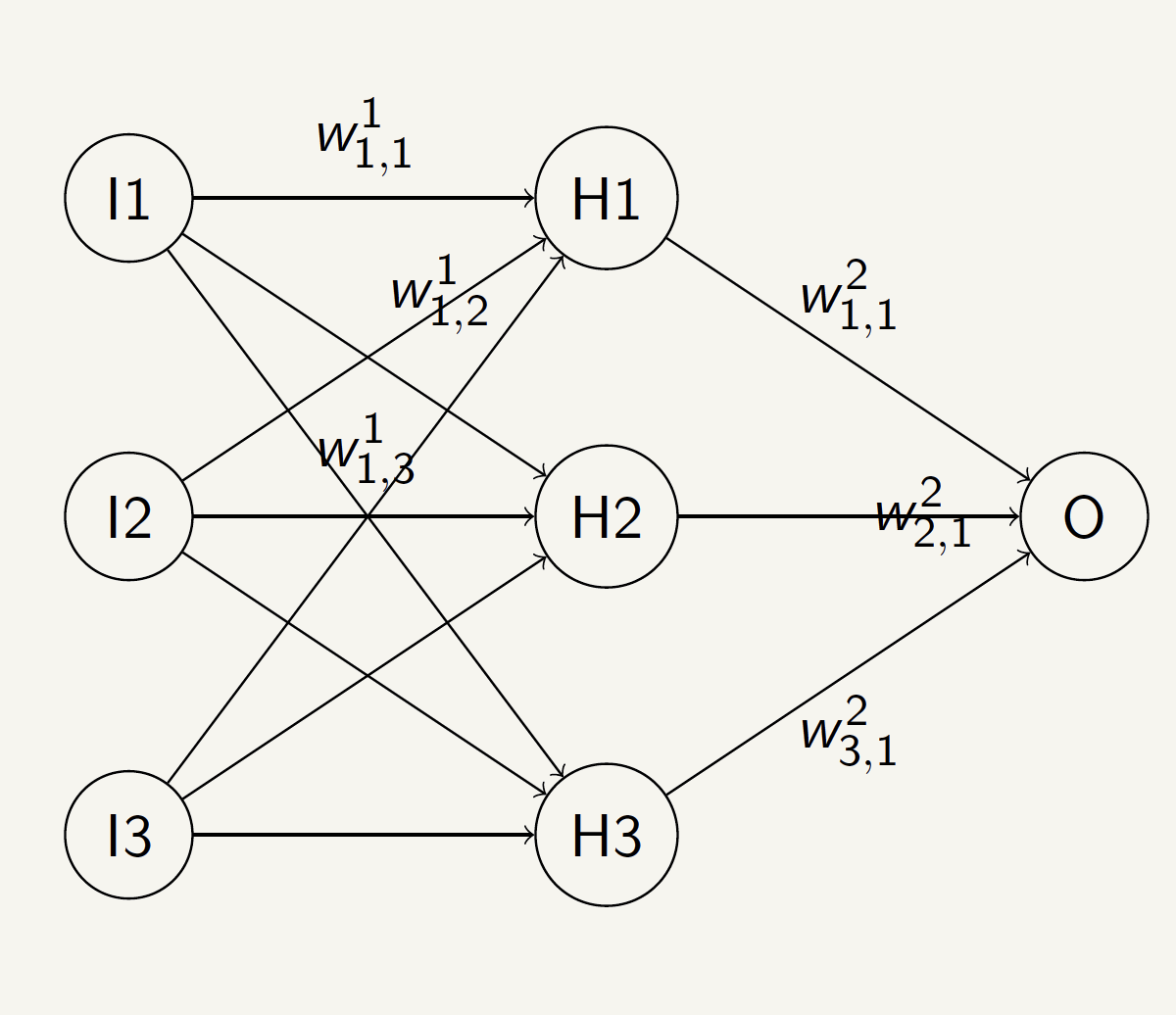
Example of a Neural Network

• For neuron (1), the weights are \(W^1_{11}, W^1_{12}, W^1_{13}\).
• For neuron (2), the weights are \(W^1_{21}, W^1_{22}, W^1_{23}\).
• For neuron (3), the weights are \(W^1_{31}, W^1_{32}, W^1_{33}\).
• Superscript \(1\) indicates the first layer.
• Subscript \(1, 2, 3\) indicates the first, second, and third neuron in the layer.

TABLE OF CONTENTS

1. Introduction✓

2. Gates Using Perceptrons✓

3. Neural Network as Computational Graph●

4. Automatic Differentiation○

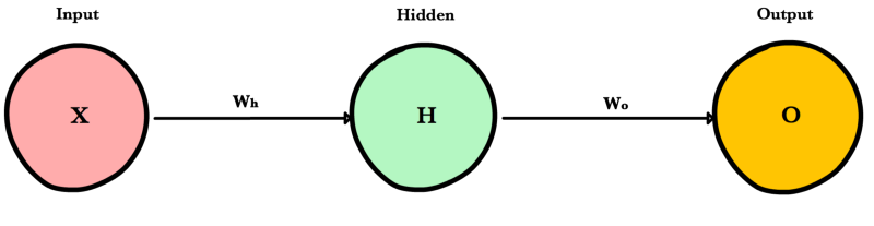
Neural Network As Computational Graph

Suppose we have a neural network with one hidden layer and one output layer to predict the probability of a house being sold given (size, bedrooms, and bathrooms)

For simplicity, no bias term and no weights for the output layer, only average:

This is a composition of functions:

This slide shows a neural network as a computational graph for house price prediction.

Computational Graph [Matrix Multiplication]

Matrix Multiplication: Training works on batches of data (e.g. 4 houses)

\[\begin{align*} \begin{bmatrix} x_1^{(1)} & x_2^{(1)} & x_3^{(1)} \\ x_1^{(2)} & x_2^{(2)} & x_3^{(2)} \\ x_1^{(3)} & x_2^{(3)} & x_3^{(3)} \\ x_1^{(4)} & x_2^{(4)} & x_3^{(4)} \end{bmatrix} \times \begin{bmatrix} w_{1,1} & w_{1,2} & w_{1,3} \\ w_{2,1} & w_{2,2} & w_{2,3} \\ w_{3,1} & w_{3,2} & w_{3,3} \end{bmatrix} = \begin{bmatrix} h_1^{(1)} & h_2^{(1)} & h_3^{(1)} \\ h_1^{(2)} & h_2^{(2)} & h_3^{(2)} \\ h_1^{(3)} & h_2^{(3)} & h_3^{(3)} \\ h_1^{(4)} & h_2^{(4)} & h_3^{(4)} \end{bmatrix} \end{align*}\] where \(x_i^{(j)}\) is feature \(i\) of house \(j\), \(w_{i,k}\) is the weight from input \(i\) to hidden node \(k\), and \(h_k^{(j)}\) is hidden node \(k\)’s value for house \(j\)

This slide demonstrates matrix multiplication in neural networks with batch processing.

Computational Graph [Sigmoid]

Sigmoid: it is applied to each element of the hidden matrix

\[\begin{align*} \begin{bmatrix} h_1^{(1)} & h_2^{(1)} & h_3^{(1)} \\ h_1^{(2)} & h_2^{(2)} & h_3^{(2)} \\ h_1^{(3)} & h_2^{(3)} & h_3^{(3)} \\ h_1^{(4)} & h_2^{(4)} & h_3^{(4)} \end{bmatrix} \rightarrow \begin{bmatrix} \sigma(h_1^{(1)}) & \sigma(h_2^{(1)}) & \sigma(h_3^{(1)}) \\ \sigma(h_1^{(2)}) & \sigma(h_2^{(2)}) & \sigma(h_3^{(2)}) \\ \sigma(h_1^{(3)}) & \sigma(h_2^{(3)}) & \sigma(h_3^{(3)}) \\ \sigma(h_1^{(4)}) & \sigma(h_2^{(4)}) & \sigma(h_3^{(4)}) \end{bmatrix} = \begin{bmatrix} a_1^{(1)} & a_2^{(1)} & a_3^{(1)} \\ a_1^{(2)} & a_2^{(2)} & a_3^{(2)} \\ a_1^{(3)} & a_2^{(3)} & a_3^{(3)} \\ a_1^{(4)} & a_2^{(4)} & a_3^{(4)} \end{bmatrix} \end{align*}\] where \(a_k^{(j)}\) is the value of activation node \(k\) for house \(j\)

This slide shows how sigmoid activation is applied element-wise to the hidden layer matrix.

Computational Graph [Average]

Average: it is applied to each row of the activation matrix

\[\begin{align*} \begin{bmatrix} a_1^{(1)} & a_2^{(1)} & a_3^{(1)} \\ a_1^{(2)} & a_2^{(2)} & a_3^{(2)} \\ a_1^{(3)} & a_2^{(3)} & a_3^{(3)} \\ a_1^{(4)} & a_2^{(4)} & a_3^{(4)} \end{bmatrix} \rightarrow \begin{bmatrix} \frac{a_1^{(1)} + a_2^{(1)} + a_3^{(1)}}{3} \\ \frac{a_1^{(2)} + a_2^{(2)} + a_3^{(2)}}{3} \\ \frac{a_1^{(3)} + a_2^{(3)} + a_3^{(3)}}{3} \\ \frac{a_1^{(4)} + a_2^{(4)} + a_3^{(4)}}{3} \end{bmatrix} \end{align*}\]

Every house now has an average probability of being sold predicted by three neurons.

This slide demonstrates how averaging is applied to compute the final output probabilities.

Chain Rule of Neural Network

What is the derivative of \(O\) with respect to \(W\)?

\(\frac{\partial O}{\partial W} = \frac{\partial U}{\partial W} \odot \frac{\partial V}{\partial U} \odot \frac{\partial O}{\partial V}\)    
Should be same shape as W, this symbol \(\odot\) is element-wise multiplication

If each computation node in the graph has a known, easy-to-compute local derivative, we can compute the derivative of the entire graph with respect to the weights using the Chain Rule

TABLE OF CONTENTS

1. Introduction✓

2. Gates Using Perceptrons✓

3. Neural Network as Computational Graph✓

4. Automatic Differentiation●

Backward Mode

Definition Backward mode computes the gradient of a final output with respect to all its intermediate inputs in a single sweep.

Mechanism It operates by traversing the transpose of the computational graph from the output node back to the input nodes using the Chain Rule.

Efficiency Highly efficient for functions with many inputs and few outputs (like neural network loss), calculating all partial derivatives simultaneously in one backward pass.

Automatic differentiation backward mode overview.

Basic Primitive Operations [Addition]

For \(z = a + b\), the gradient of \(z\) with respect to \(a\) is 1, and with respect to \(b\) is 1.

Basic Primitive Operations [Subtraction]

For \(z = a - b\), the gradient of \(z\) with respect to \(a\) is 1, and with respect to \(b\) is -1.

Basic Primitive Operations [Multiplication]

For \(z = a * b\), the gradient of \(z\) with respect to \(a\) is \(b\), and with respect to \(b\) is \(a\).

Basic Primitive Operations [Division]

For \(z = a / b\), the gradient of \(z\) with respect to \(a\) is \(\frac{1}{b}\), and with respect to \(b\) is \(-\frac{a}{b^2}\).

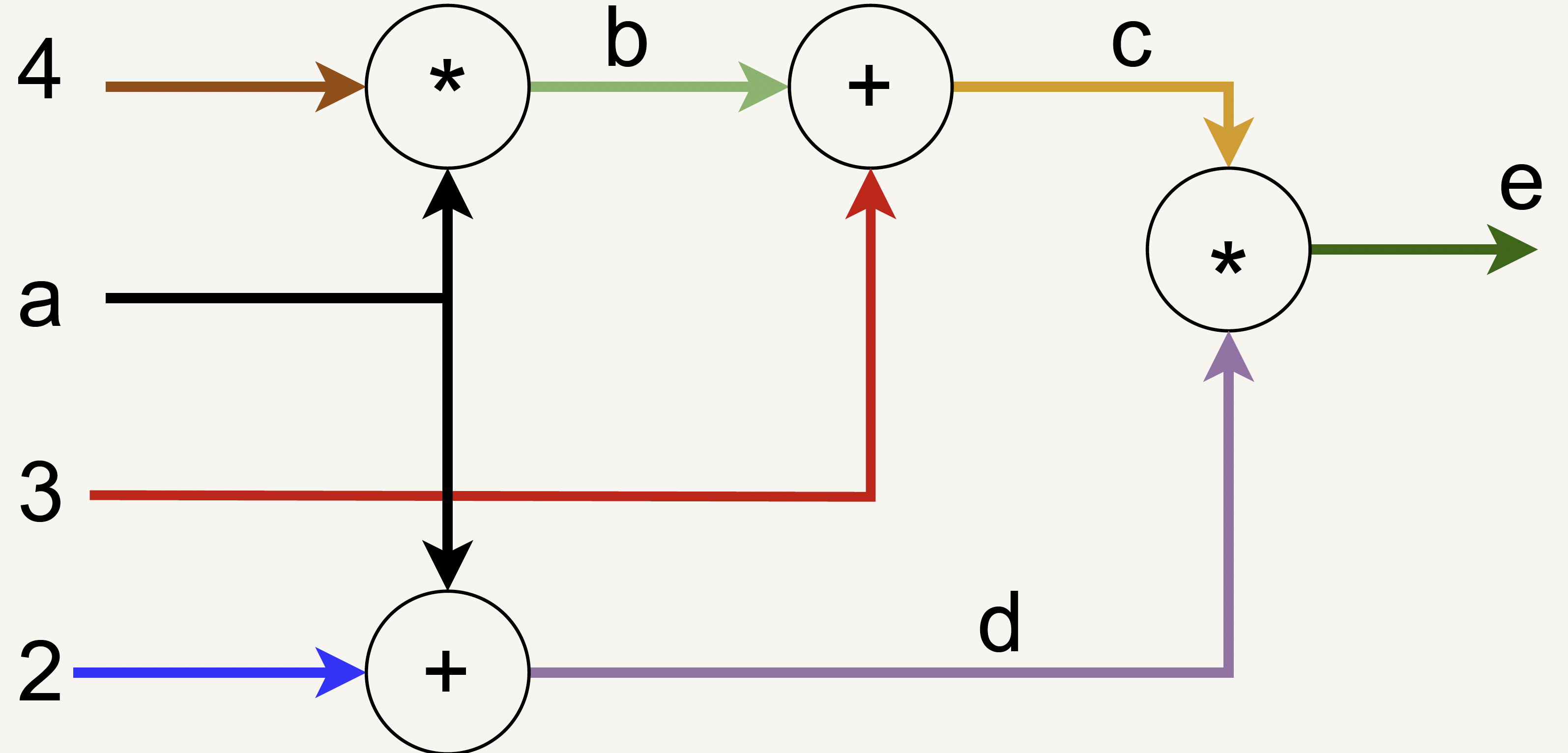
Backward Mode Computational Graph Example

Suppose we have the following equation:

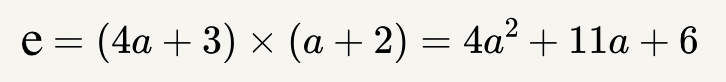
What is \(\frac{\partial e}{\partial a}\) at \(a=3\)?

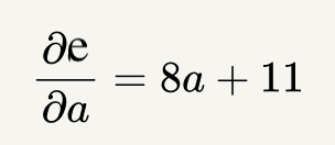
Derivative Example

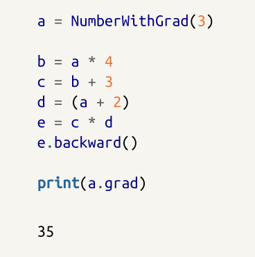
Derivative Example

\(\frac{\partial e}{\partial e} = 1\)

\(\frac{\partial e}{\partial c} = d = 5\)

\(\frac{\partial e}{\partial d} = c = 15\)

\(\frac{\partial e}{\partial b} = 5 \cdot 1 = 5\)

\(5 \cdot 4 = 20\)

\(15 \cdot 1 = 15\)

\(\frac{\partial e}{\partial a} = 20 + 15 = 35\)

Simple Autograd Implementation [1/2]

from typing import Union, List

Numberable = Union[float, int]

def ensure_number(num: Numberable):
    if isinstance(num, NumberWithGrad):
        return num
    else:
        return NumberWithGrad(num)        

class NumberWithGrad(object):
    def __init__(self, num: Numberable, depends_on: List[Numberable] = None, creation_op: str = ''):
        self.num = num
        self.grad = None
        self.depends_on = depends_on or []
        self.creation_op = creation_op

    def __add__(self, other: Numberable):
        return NumberWithGrad(self.num + ensure_number(other).num,
                              depends_on = [self, ensure_number(other)],
                              creation_op = 'add')
    
    def __mul__(self, other: Numberable = None):
        return NumberWithGrad(self.num * ensure_number(other).num,
                              depends_on = [self, ensure_number(other)],
                              creation_op = 'mul')

Simple Autograd Implementation [2/2]

    def backward(self, backward_grad: Numberable = None):
        if backward_grad is None: # first time calling backward
            self.grad = 1
        else: 
            # Accumulate gradient
            if self.grad is None:
                self.grad = backward_grad
            else:
                self.grad += backward_grad
        
        if self.creation_op == "add":
            # Send backward self.grad
            self.depends_on[0].backward(self.grad)
            self.depends_on[1].backward(self.grad)    

        if self.creation_op == "mul":
            # Calculate derivative w.r.t first element
            new = self.depends_on[1] * self.grad
            self.depends_on[0].backward(new.num)

            # Calculate derivative w.r.t second element
            new = self.depends_on[0] * self.grad
            self.depends_on[1].backward(new.num)

Autograd Example Usage

Let’s test our NumberWithGrad class:

a = NumberWithGrad(3)
b = a * 4
c = b + 3

c.backward()

print("Gradients:")
print("a.grad:", a.grad) # Expected: 4
print("b.grad:", b.grad) # Expected: 1

Thank You!